Any design involving ignition coils more sophisticated than the very simplest will require some detailed knowledge of the characteristics of the ignition coil that will be used in the design. Detailed datasheets with thorough characterization and key parameters are unlikely to be available, but many of these values can be obtained with relatively simple equipment and techniques. Some designs may require more detail than others, so the most basic specifications are determined first, and an increasingly detailed model is developed. The structure of the ignition coil is very similar to that of a standard transformer, and most of the modelling and measurement techniques are valid for both. In both cases, the most basic parameter is the turns ratio of the coils. There is a fairly typical range for the turns ratio of ignition coils, generally between perhaps 50:1 to 200:1, with 100:1 probably being the most common. Measurements that indicate a turns ratio significantly outside of this range may indicate an error in measurement or a damaged coil. The simplest method to measure the turns ratio is to apply an AC voltage to one coil, and compare the magnitude of the voltage at the other coil. The main concern with making this measurement is to be careful of the magnitude of the applied AC signal. Applying a too large of a singal may have several effects. First, applying too large of a volt-second product will result in the core saturating resulting in incorrect results. Also, If the magnetizing current resulting from a large volt-second product becomes too large and the voltage source's impedance is high (such as with a function generator) the output may saturate resulting in clipping and erroneous measurements. Keeping those considerations in mind, the actual measurement is very simple. 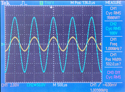 Fig. 1: Measurement of Ignition Coil Turns Ratio Using these measurements, the turns ratio is calculated as the RMS value of the high voltage coil divided by the RMS value of the low voltage coil. Dividing 100 V by 983 mV results in a turns ratio of 101.7, very nearly 100:1. The model so far looks like 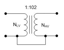 Fig. 2: Ignition Coil Model, Turns Ratio In addition to the ideal transformer action measured above, their is also an inductance in parallel with the ideal transformer which is called the magnetizing inductance. Typically, the magnetizing inductance is shown on the primary side of the transformer; however, it can be reflected to any winding by the square of the turns ratio. The magnetizing inductance is the inductance that is measured at the transformer terminals. The most straightforward method of measuring the magnetizing inductance is by using an inductance meter, but a function generator, resistor, and oscilloscope can also be used. I measured the magnetizing inductance of my coil with an LCR meter and got 5.5 mH at the primary winding and 57.2 H at the secondary. Note that these two measurements are measuring the same element in the circuit - there aren't two independent elements being measured. As evidence of this, dividing the secondary measured inductance by the turns ratio squared, i.e. 57.2 H divided by 1022, yields almost exactly 5.5 mH. 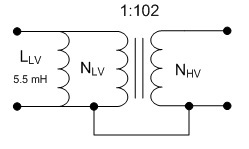 Fig. 3: Ignition Coil Model, Magnetizing Inductance Included These measurements can be used to double check the turns ratio measurement made earlier as well. The inductance of each coil is given by 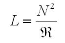 Eq. 1: Inductance of a Coil where N is the number of turns and  is the
reluctance of the core. By solving for reluctance we obtain is the
reluctance of the core. By solving for reluctance we obtain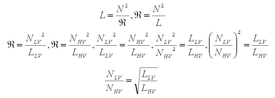 Eq. 2: Re-arranged equations Using the values measured earlier, the turns ratio is computed to be 102:1 by Eq. 2 as well, which supports the initial calculation. The next refinement of the model is to add the leakage inductances. The leakage inductance represents the flux through one coil which is not linked to the other coil, and is modeled as an inductance in series with the magnetizing inductance. More specifically, the leakage flux is the portion of the measured magnetizing inductance which is not linked to the other coil, so the measured leakage inductance is subtracted from the self-inductance to obtain a better estimation. Consider an ideal transformer with a shorted secondary. In this configuration, the impedance of the primary can be computed as the impedance of the secondary multiplied by the turns ratio squared. With a shorted secondary (i.e. the secondary's impedance is zero) the impedance of the primary would also be zero. 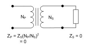 Fig. 4: Transformer with Shorted Secondary If the secondary is shorted on a practical transformer and the impedance is measured at the primary the result will show some finite value of inductance is present. This is due to the leakage inductance, which is not linked to the secondary, and therefore does not represent the secondary's scaled impedance. 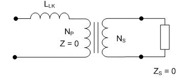 Fig. 5: Transformer with Leakage Inductance Using this method, the leakage inductance for the low and high voltage coils were measured to be 612 uH and 6.76 H, respectively. Adding these leakage inductances to the model results in 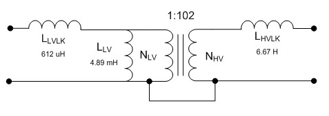 Fig. 6: Ignition Coil Model with Leakage Inductances Included So far the model has only taken into consideration purely inductive effects; however, at higher frequencies capacitive behavior becomes dominant. This is usually attributed to the capacitance between windings, but these capacitances do not entirely explain the behavior observed. Simply, the lumped model that is used to describe the inductance becomes inadequate as the wavelengths become shorter and comparable in length to the coil itself. At some point, as the frequency is increased, the inductive and capacitive reactances cancel and the coil will resonate. This point is called the self resonant frequency. The lumped model can be modified with the addition of a capacitor to correct its behavior over a limited range of frequencies above the self-resonant frequency without resorting to a transmission line model. Determining the self-resonant frequency is aided by the fact that the coil appears completely resistive at this frequency. At this point the voltage and current through a coil will be in phase, allowing the self-resonant frequency to be determined by sweeping the frequency and noting the point at which the voltage and current are in phase. 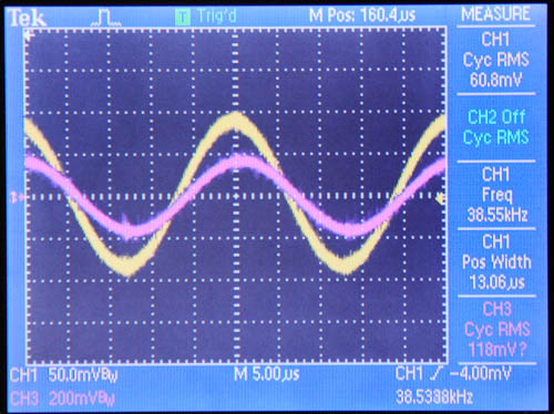 Fig. 7: Determining Self-Resonant Frequency Here, the self-resonant frequency for my coil is determined to be 38.55 kHz. The relationship between resonance and frequency for a parallel LC circuit is 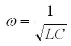 Eq. 3: Resonant Frequency of a Parallel LC Circuit Solving this equation for the capacitance gives the result 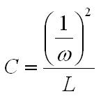 Eq. 4: Determining Resonant Capacitance Using the self-inductance of the low voltage winding and the self-resonant frequency, the resonant capacitance can be calculated to be 3.49 nF. The model with this capacitance is shown below. 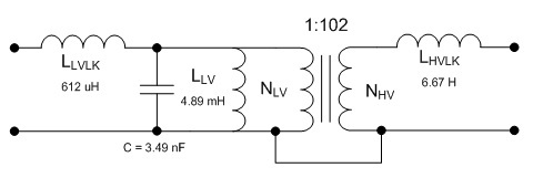 Fig. 8: Ignition Coil with Capacitance Included In addition to the inductive and capacitive elements already discussed, the copper windings also have some resistance. These values can be easily measured with an Ohm meter. I determined the low voltage and high voltage coil resistances to be 1.7 and 8.7 kOhms respectively. It's tempting to use the values directly in the model; however, these values are seldom accurate at high frequencies. This is somewhat counter intuitive, since resistance is generally not considered to be frequency dependant. In the case of resistance at high frequencies two effects, called the skin and proximity effect, can greatly increase the resistance to AC signals. The skin effect causes ac currents of increasing frequency to penetrate less deeply into a conductor from the surface. This reduces the cross section through which the current flows, and consequently increases the resistance. The skin depth, or effective depth that currents penetrate is give by the equation 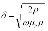 Eq. 5: Skin Depth where  is the skin depth,
  is the
resistivity of the conductor ( is the
resistivity of the conductor ( for copper) and for copper) and  is the
permeability of free space (equal to is the
permeability of free space (equal to  for
most non-magnetic materials) and for
most non-magnetic materials) and  is the
relative permeability of the conductor (approximately 1 for most
non-ferrous conductors.) The resistance of a length of a wire with
a given length and cross sectional area can be computed by is the
relative permeability of the conductor (approximately 1 for most
non-ferrous conductors.) The resistance of a length of a wire with
a given length and cross sectional area can be computed by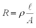 Eq. 6: Resistance where  is
the length of the conductor and is
the length of the conductor and  is the cross section of the conductor. If the diameter of the wire is
less than twice the skin depth, then the area can be computed
using
is the cross section of the conductor. If the diameter of the wire is
less than twice the skin depth, then the area can be computed
using  .
Otherwise, the cross section of the conductive region will be smaller
and should be computed as shown in Fig. 9. .
Otherwise, the cross section of the conductive region will be smaller
and should be computed as shown in Fig. 9.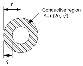 Fig. 9: Area of Conduction for a Cylindrical Conductor Therefore, the resistance of a length of wire where the diameter is smaller than the skin depth is given by 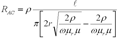 Eq. 7: AC Resistance of a Wire with Skin Effect The proximity effect occurs when a winding is more than one layer thick, and is the result of the changing magnetic flux from the previous layer cancelling out the current on the interior of the current winding and increasing the current on the outside of the winding. The effect is compounded with each additional layer in a coil, and can greatly increase the effective AC resistance. Proximity
Fig. 10: Proximity Effect The exact form for the proximity effect is beyond the scope of this discussion, so the combined effect of the skin and proximity effect are combined to shown their cumulative effect on AC resistance. 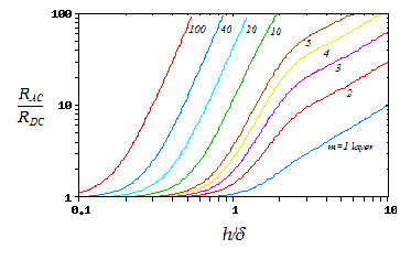 Fig. 11: Dowell Plot This graph, known as a Dowell plot, can be used to calculate the factor by which the DC resistance should be multiplied in order to determine the AC resistance. The X axis is the height of the conductor divided by the skin depth at the frequency of interest, and is followed vertically until it intersects the curve for the number of layers in the coil. This point's position is then noted on the vertical axis, and the resistance multiplier is read off. As an example, a coil made of a conductor with a ratio of height to skin depth of three and two layers of windings has an AC resistance about 12 times higher thant the DC resistance of the wire. It should be noted that these curves are derived for sinusoidal waveforms at a given frequency. Switching waveforms contain frequencies at the fundamental and higher harmonics, so depending on the waveform the actual resistance may be perhaps 1.2 to 2 times higher than indicated by the Dowell plot. If you happen to know the construction specifics of your ignition coil you can estimate the AC resistance using this method. More than likely you won't have access to that information unless you disassemble and destroy the coil, which is most likely unecessary. The AC resistance for a given switching frequency can be determined by simple measurement with enough fidelity for this model. Assuming a switching frequency of 100 Hz, the low voltage and high voltage winding resistances were measured as 9.78 Ohms and 9.38 kΩ respectively (compared to 1.7 Ω and 8.7 kΩ at DC.) The model, including the winding resistances at 100 Hz is shown in Fig. 12. 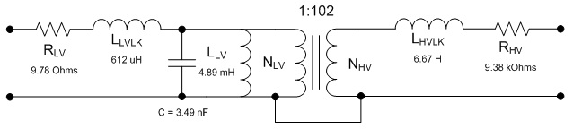 Fig. 12: Ignition Coil Model with Coil Resistances Included [ Back to Ignition Coils ] [ Back to Main ] Questions?
Comments? Suggestions? E-Mail me at MyElectricEngine@gmail.com
Copyright 2007-2010 by Matthew Krolak - All Rights Reserved. Don't copy my stuff without asking first. |